1. Quick Study of Deep Learning¶

Optimization Algorithms¶

Stochastic Gradient Descent (SGD) updates parameters using a subset (batch) of the data to compute the gradient, which helps in overcoming the computational challenges of handling large datasets: $w_{t+1} = w_t - \eta \cdot g_t$ , where
- $w_t$ is the parameter vector at step $t$
- $\eta$ is the learning rate
- $g_t = \nabla L(w_t)$ is the gradient of the loss function $L$ with respect to $w_t$ averaged over a batch.
ADAM (Adaptive Moment Estimation) computes adaptive learning rates for each parameter:

$m_t &= \beta_1 m_{t-1} + (1 - \beta_1) \cdot g_t \\ v_t &= \beta_2 v_{t-1} + (1 - \beta_2) \cdot g_t^2 \\ \hat{m}_t &= \frac{m_t}{1 - \beta_1^t} \\ \hat{v}_t &= \frac{v_t}{1 - \beta_2^t} \\ w_{t+1} &= w_t - \frac{\eta}{\sqrt{\hat{v}_t} + \epsilon} \cdot \hat{m}_t$

where
- $m_t$ and $v_t$ are the moving averages of the gradients and squared gradients.
- $\beta_1$ and $\beta_2$ are the decay rates for these moving averages.
- $\eta$ is the learning rate.
- $\epsilon$ is a small scalar used to prevent division by zero.
- $g_t$ represents the gradient at time step $t$ .

ADAM could converge faster than SGD because it adjusts the learning rate dynamically for each parameter based on estimates of first and second moments of the gradients. ADAM is often easier to tune due to its adaptive nature. SGD often leads to better generalization on unseen data. So some researchers leverage the fast convergence of Adam in the early phase and switch to SGD in later stages of training.

Deep Learning Frameworks¶

PyTorch is a flexible deep learning framework that allows dynamic computation graphs and is particularly loved for its ease of use and simplicity in defining complex models.
TensorFlow is another widely used library that offers both flexibility and scalability in building and deploying deep learning models, especially suited for production environments.

Next, we review some standard learning problems along with examples to get you started. You can copy and paste these into your notebooks to try them out.

Supervise Learning¶

Supervised learning is a type of machine learning where a model is trained on a labeled dataset, learning to predict output labels from input features. The model’s performance is measured against known labels to improve its accuracy over time.

For a practical example, let us train a simple logistic regression model for image classification using CIFAR-10 dataset, which consists of images categorized into 10 different classes. each image has dimensions of 32x32 pixels, and since these images are in color, each has 3 color channels (Red, Green, Blue). Therefore, each image has a total of 32×32×3=3072 pixels.

Logistic Model¶

First install and import some packages.

import numpy as np
import matplotlib.pyplot as plt
from sklearn.linear_model import LogisticRegression
from sklearn.model_selection import train_test_split
from sklearn.metrics import accuracy_score
import torch
import torch.nn as nn
import torch.optim as optim
from torchvision import datasets, transforms, models
from torch.utils.data import DataLoader
from sklearn.linear_model import SGDClassifier
from sklearn.manifold import TSNE
import time

Load CIFAR-10 data.

transform = transforms.Compose([
    transforms.ToTensor(),  # Converts to [0, 1] interval.
    transforms.Lambda(lambda x: x.view(-1))  # Flatten the image
])
train_dataset = datasets.CIFAR10(root='./data', train=True, download=True, transform=transform)
test_dataset = datasets.CIFAR10(root='./data', train=False, download=True, transform=transform)

# DataLoader for batch processing
batch_size = 5000  # Adjust based on memory capacity
train_loader = DataLoader(train_dataset, batch_size=batch_size, shuffle=True)
test_loader = DataLoader(test_dataset, batch_size=batch_size, shuffle=False)

# CIFAR-10 class names
class_names = ['airplane', 'automobile', 'bird', 'cat', 'deer', 'dog', 'frog', 'horse', 'ship', 'truck']

Initialize the logistic regression model with elastic net penalty using SGDClassifier

model = SGDClassifier(loss='log_loss', penalty='elasticnet', l1_ratio=0.5, max_iter=100, tol=1e-3, verbose=0)

Prepare for logging.

def evaluate_model(model, test_loader):
    y_true, y_pred = [], []
    for images, targets in test_loader:
        y_pred.extend(model.predict(images.numpy()))
        y_true.extend(targets.numpy())
    return accuracy_score(y_true, y_pred), y_pred

def visualize_predictions(y_pred, test_loader, class_names):
    fig, axes = plt.subplots(1, 5, figsize=(10, 2))
    test_images = test_loader.dataset.data[:5]  # Get the first 5 images from the test dataset
    test_labels = [class_names[label] for label in y_pred[:5]]
    for ax, img, label in zip(axes, test_images, test_labels):
        ax.set_title(f'Pred: {label}')
        ax.imshow(img)
        ax.axis('off')
    plt.show()
    plt.close(fig)  # Close the figure to free up memory

Now, we train the model and keep monitoring the test performance.

for epoch in range(4):  # Number of epochs
    for images, targets in train_loader:
        model.partial_fit(images.numpy(), targets.numpy(), classes=np.unique(train_dataset.targets))
    if (epoch + 1) % 2 == 0:  # Log every 2 epochs
        print(f'-- Epoch {epoch + 1}')
        print(f'Norm: {np.linalg.norm(model.coef_)}, Bias: {model.intercept_[0]}')
        accuracy, y_pred = evaluate_model(model, test_loader)
        print(f'Accuracy: {accuracy}')
        visualize_predictions(y_pred, test_loader, class_names)

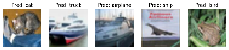
In a particular run, we got the test accuracy of 0.30 after 4 epochs, with the following randomly selected images and their prediction results for demo.

Figure: A Snapshot of Logistic Regression for CIFAR10 at 4 epochs

Sample Predictions

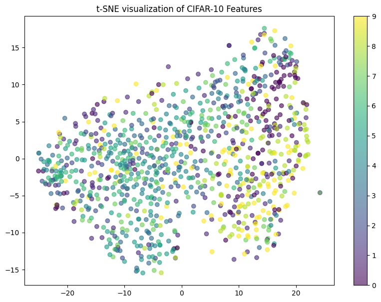
The low accuracy is not surprising if we visualize the data in 2D:

X_visual, y_visual = next(iter(train_loader))
X_visual_tsne = TSNE(n_components=2, random_state=42).fit_transform(X_visual.numpy()[:500])

# Visualize using t-SNE
plt.figure(figsize=(10, 7))
plt.scatter(X_visual_tsne[:, 0], X_visual_tsne[:, 1], c=y_visual.numpy()[:500], cmap='viridis', alpha=0.6)
plt.colorbar()
plt.title('t-SNE visualization of CIFAR-10 Features')
plt.show()

The result will be something like the following. Clearly, it is unrealistic to well separate classes using linear decision boundaries.

Figure: 2D visualization of CIFAR10 data

2D visual

ResNet Model {#resnet-model}¶

Now suppose we will use a deep neural network, particularly a ResNet model, to train a classifier from scratch.

Prepare for logging.

def print_epoch_stats(epoch, running_loss, train_loader, start_time, end_time):
    print(f'Epoch {epoch+1}, Loss: {running_loss/len(train_loader)}, Time: {end_time - start_time}s')

def evaluate_model(model, device, test_loader):
    model.eval()  # Set the model to evaluation mode
    y_true = []
    y_pred = []
    with torch.no_grad():  # Turn off gradients for validation, saves memory and computations
        for images, labels in test_loader:
            images, labels = images.to(device), labels.to(device)
            outputs = model(images)
            _, predicted = torch.max(outputs, 1)
            y_pred.extend(predicted.cpu().numpy())
            y_true.extend(labels.cpu().numpy())
    accuracy = accuracy_score(y_true, y_pred)
    return accuracy, y_pred

def visualize_predictions(images, predicted, class_names):
    fig, axes = plt.subplots(1, 5, figsize=(10, 2))
    for ax, img, pred in zip(axes, images, predicted):
        img = img.permute(1, 2, 0)  # Convert from CxHxW to HxWxC for matplotlib
        ax.imshow(img)
        ax.set_title(f'Pred: {class_names[pred]}')
        ax.axis('off')
    plt.show()			

Train a ResNet18 model to classifier 32x32 image inputs from scratch.

model = models.resnet18(pretrained=False)
model.conv1 = nn.Conv2d(3, 64, kernel_size=3, stride=1, padding=1, bias=False)  # Change the first conv layer
model.maxpool = nn.Identity()  # Omit max pooling
model.fc = nn.Linear(model.fc.in_features, 10)  # Adjust for number of classes

# Data loaders
transform = transforms.Compose([
    transforms.ToTensor(),  # Convert to tensor
    transforms.Normalize((0.5, 0.5, 0.5), (0.5, 0.5, 0.5))  # Normalize the data
])
train_loader = torch.utils.data.DataLoader(
    datasets.CIFAR10('./data', train=True, download=True, transform=transform),
    batch_size=64, shuffle=True)
test_loader = torch.utils.data.DataLoader(
    datasets.CIFAR10('./data', train=False, download=True, transform=transform),
    batch_size=5, shuffle=False)

# CIFAR-10 class names
class_names = ['airplane', 'automobile', 'bird', 'cat', 'deer', 'dog', 'frog', 'horse', 'ship', 'truck']

# Check for GPU availability and define device
device = torch.device("cuda" if torch.cuda.is_available() else "cpu")
print(f"Using {device}")
model = model.to(device)

# Training settings
optimizer = optim.Adam(model.parameters(), lr=0.001)
criterion = nn.CrossEntropyLoss()

# Training loop
for epoch in range(4):
    start_time = time.time()
    model.train()
    running_loss = 0.0
    for i, (inputs, labels) in enumerate(train_loader):
        inputs, labels = inputs.to(device), labels.to(device)
        optimizer.zero_grad()
        outputs = model(inputs)
        loss = criterion(outputs, labels)
        loss.backward()
        optimizer.step()
        running_loss += loss.item()

    end_time = time.time()
    print_epoch_stats(epoch, running_loss, train_loader, start_time, end_time)

    # Visualization every 2 epochs
    if (epoch + 1) % 2 == 0:
        model.eval()
        with torch.no_grad(): 
            accuracy, _ = evaluate_model(model, device, test_loader)
            print(f'Accuracy: {accuracy}')

            images, labels = next(iter(test_loader))
            images, labels = images.to(device), labels.to(device)
            outputs = model(images)
            _, predicted = torch.max(outputs, 1)
            predicted = predicted.cpu().numpy()
            images = images.cpu()
            visualize_predictions(images, predicted, class_names)

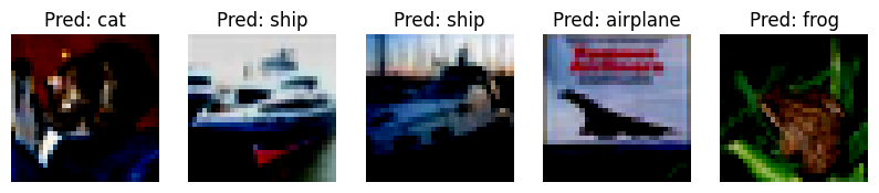
In a particular run, we got the test accuracy of 0.75 after 4 epochs, with the following randomly selected images and their prediction results for demo.

Figure: A Snapshot of ResNet for CIFAR10 at 4 epochs

Sample Predictions

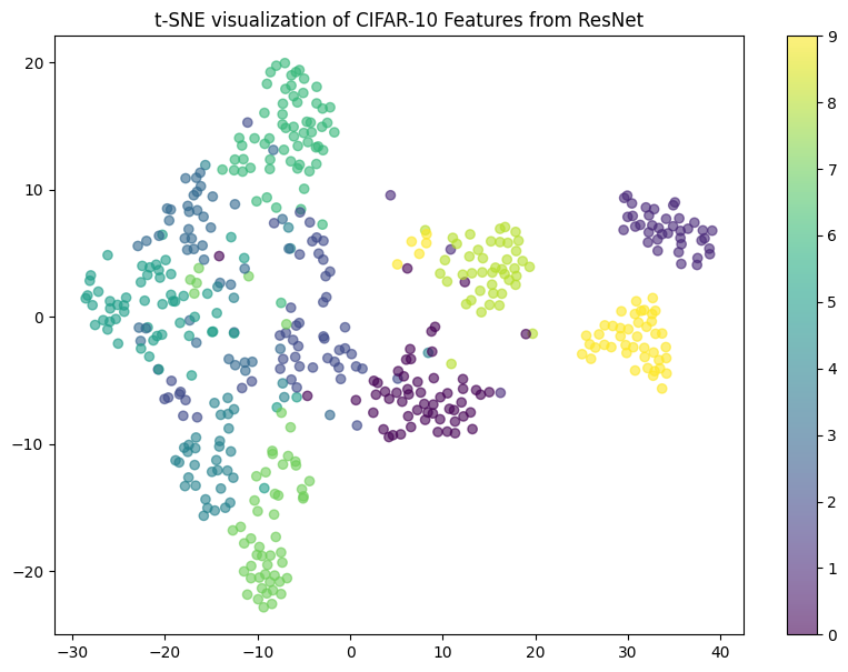
The reasonably high accuracy is not surprising if we visualize the feature outputs from the second-last layer in 2D which seem to be almost linearly separable.

def extract_features_and_visualize(model, device, data_loader):
    # Modify the model to output features from the last layer before the fully connected layer
    model_modified = torch.nn.Sequential(*(list(model.children())[:-1]))
    model_modified = model_modified.to(device)
    
    # Extract features
    features = []
    labels = []
    with torch.no_grad():
        for images, targets in data_loader:
            images = images.to(device)
            output = model_modified(images)
            output = output.view(output.size(0), -1)  # Flatten the outputs
            features.append(output.cpu().numpy())
            labels.append(targets.numpy())

    features = np.concatenate(features)
    labels = np.concatenate(labels)

    # t-SNE transformation
    tsne = TSNE(n_components=2, random_state=42)
    features_tsne = tsne.fit_transform(features[:500])  # Using subset for manageability

    # Visualization
    plt.figure(figsize=(10, 7))
    plt.scatter(features_tsne[:, 0], features_tsne[:, 1], c=labels[:500], cmap='viridis', alpha=0.6)
    plt.colorbar()
    plt.title('t-SNE visualization of CIFAR-10 Features from ResNet')
    plt.show()

# evaluate the earlier trained model
extract_features_and_visualize(model, device, train_loader)

The result will be something like the following.

Figure: 2D visualization of CIFAR10 data under a trained ResNet18

2D visual

Computation Resource Management¶

Deep learning computations can be extremely resource-intensive. Accelerating these computations is crucial, particularly using Graphics Processing Units (GPUs): Optimized for parallelizing matrix operations in deep learning.

CPU vs GPUs: CPUs are generally used for tasks that require less parallel computation, such as data preprocessing or running the training loop itself. GPUs, on the other hand, are optimized for highly parallelizable tasks like matrix multiplications in training neural networks. A typical workflow:
Minibatching In training large models under limited GPU memory, minibatching processes small subsets of the dataset at a time, and accumulates gradients over multiple forward passes before performing a backpropagation step. Basically, it simulates a larger batch size without exceeding memory limits.

Using the earlier example, Let’s analyze the performance difference between CPU and GPU.

Exercises

We expect a larger benefit of using GPU especially as the network complexity increases, e.g., more layers or larger batch sizes, due to the GPU’s ability to parallelize operations more efficiently than a CPU. Redo the earlier experiments to compare CPU and GPU.

Unsupervised Learning¶

Unsupervised Learning aims to understand the underlying structure of the data without explicit labels. Variational Autoencoders (VAEs) are a type of generative model often used in unsupervised learning. They encode data into a condensed latent space and then decode it back to the original space, which can be understood as a nonlinear generalization of PCA.

Variational Autoencoder (VAE)¶

An example VAE architecture is given as follows, assuming the inputs are 784-dimensional data (28x28 images from MNIST).

import torch
import torch.nn as nn
import torch.optim as optim
from torchvision import datasets, transforms

class VAE(nn.Module):
    def __init__(self):
        super(VAE, self).__init__()
        self.fc1 = nn.Linear(784, 400)
        self.fc21 = nn.Linear(400, 20)  # mu layer
        self.fc22 = nn.Linear(400, 20)  # log variance layer
        self.fc3 = nn.Linear(20, 400)
        self.fc4 = nn.Linear(400, 784)

    def encode(self, x):
        h1 = torch.relu(self.fc1(x))
        return self.fc21(h1), self.fc22(h1)

    def reparameterize(self, mu, logvar):
        std = torch.exp(0.5 * logvar)
        eps = torch.randn_like(std)
        return mu + eps * std

    def decode(self, z):
        h3 = torch.relu(self.fc3(z))
        return torch.sigmoid(self.fc4(h3))

    def forward(self, x):
        mu, logvar = self.encode(x.view(-1, 784))
        z = self.reparameterize(mu, logvar)
        return self.decode(z), mu, logvar

# Training settings
batch_size = 1024
epochs = 10
learning_rate = 1e-3

# Data loader
train_loader = torch.utils.data.DataLoader(
    datasets.MNIST('../data', train=True, download=True, transform=transforms.ToTensor()),
    batch_size=batch_size, shuffle=True)
    
# Check for GPU availability and set the device
device = torch.device("cuda" if torch.cuda.is_available() else "cpu")
print(f"Using {device}")

# Initialize the model and send it to the device
model = VAE().to(device)
optimizer = optim.Adam(model.parameters(), lr=learning_rate)

Encoder Network: This part of the VAE maps the input into a latent space. In the code, fc1 is the first layer of the encoder that reduces the dimension from the flattened 784 pixels to 400. Then, fc21 and fc22 further map these 400 dimensions to two different 20-dimensional outputs: one for the means (mu) and one for the logarithm of the variances (logvar). These represent the parameters of the Gaussian distribution from which the latent variables are sampled.
Decoder Network: This network maps the latent space back to the original data space. In your code, fc3 and fc4 perform this task, with fc3 mapping the 20-dimensional latent vectors back up to 400 dimensions and fc4 reconstructing the original 784-dimensional output.

Everything is in place except for the loss function needed for training. But how do we define the loss so that we get a reasonable encoder-decoder model that approximates the underlying distribution of the data, denoted as $p(x)$ ?

From ELBO to VAE Loss¶

Let’s take a step back and consider a more general framework, not limited to the VAE architecture above. Suppose we aim to map the data $x$ to some (often low-dimensional) latent variable $z$ (also referred to as the “code”) and then map it back to $x$ . Let $q_{\phi}(z \mid x)$ represent the parameterized encoder, and for now, we set aside the decoder. We can derive that, for any $q_{\phi}$ ,

$\log p(x) & =\mathbb{E}_{q_{\phi}(z \mid x)}[\log p(x)] \\ & =\mathbb{E}_{q_{\phi}(z \mid x)}\left[\log \frac{p(x, z) }{p(z \mid x)} \cdot \frac{q_{\phi}(z \mid x)}{q_{\phi}(z \mid x)}\right] \\ & =\mathbb{E}_{q_{\phi}(z \mid x)}\left[\log \frac{q_{\phi}(z \mid x)}{p(z \mid x)}\right] + \mathbb{E}_{q_{\phi}(z \mid x)}\left[\log \frac{p(x, z)}{q_{\phi}(z \mid x)}\right] \\ & = D_{\mathrm{KL}}\left(q_{\phi}(z \mid x) \| p(z \mid x)\right) + \mathbb{E}_{q_{\phi}(z \mid x)}\left[\log \frac{p(x, z)}{q_{\phi}(z \mid x)}\right].$

The left hand side does not involve $q_{\phi}$ . The right hand consists of two terms. The first term is more interpretable. It is a KL divergence term that measures the deviation of the modeled posterior (treating as $z$ as the parameter of interest under a specified model) from the true, unknown posterior $p(z \mid x)$ . Therefore, it becomes a reasonable objective to minimize this term so that we obtain as an as accurate code as possible. But $p(z \mid x)$ looks more difficult to obtain compared with $p(x,z) = p(z) p(x \mid z)$ , so in practice we often maximize the second term, also known as the Evidence Lower Bound (ELBO).

Why ELBO is relatively easier to approximate? Since $p(x,z) = p(z) p(x \mid z)$ , we can specify $p(z)$ as the prior distribution and learn the parameterized $p_{\theta}(x \mid z)$ , which directly corresponds to a decoder model. In summary, we now turn the modeling of a generative distribution of $x$ into the objective of

$\max_{\phi, \theta} \mathbb{E}_{q_{\phi}(z \mid x)}\left[\log \frac{p(z) p_{\theta}(x \mid z)}{q_{\phi}(z \mid x)}\right] = - D_{\mathrm{KL}}\left(q_{\phi}(z \mid x) \| p(z)\right) + \mathbb{E}_{q_{\phi}(z \mid x)} \log p_{\theta}(x \mid z)$

or equivalently,

$\min_{\phi, \theta} \textrm{loss}(x) = \textrm{loss}_{\textrm{Encoder}}(x) + \textrm{loss}_{\textrm{Decoder}}(x),$

where $\textrm{loss}_{\textrm{Encoder}}(x) = D_{\mathrm{KL}}\left(q_{\phi}(z \mid x) \| p(z)\right)$ aims to regularize the posterior of the code not too far from the prior distribution, and $\textrm{loss}_{\textrm{Decoder}}(x) = -\mathbb{E}_{q_{\phi}(z \mid x)} \log p_{\theta}(x \mid z)$ aims to reduce the reconstruction error.

Going back to VAE case, in line with the above general loss, the VAE loss is the sum of:

KL Divergence
BCE (Binary Cross-Entropy)

We give a concrete derivation of the KL Divergence in VAE case. Suppose the standard Normal distribution is used for the prior distribution $p(z)$ . It is calculated that for two Normal distributions $\mathcal{N}_0(\mu_0, \sigma_0^2)$ and $\mathcal{N}_1(\mu_1, \sigma_1^2)$ , the KL divergence is

$D_{KL}(\mathcal{N}_0 \| \mathcal{N}_1) = \log\frac{\sigma_1}{\sigma_0} + \frac{\sigma_0^2 + (\mu_0 - \mu_1)^2}{2\sigma_1^2} - \frac{1}{2}$

For a VAE, where $q(z \mid x)$ is approximated by $\mathcal{N}(z; \mu, \sigma^2)$ and $p(z) = \mathcal{N}(z; 0, I)$ , we have $\mu_0 = \mu$ , $\sigma_0 = \sigma = \exp\left(\frac{1}{2} \log \sigma^2\right)$ , $\mu_1 = 0$ , $\sigma_1 = 1$ . Therefore,

$D_{\mathrm{KL}}(q(z|x) \| p(z)) &= \log\frac{1}{\sigma} + \frac{\sigma^2 + \mu^2}{2} - \frac{1}{2} \\ &= -\frac{1}{2} (1 + \log \sigma^2 - \mu^2 - \exp(\log \sigma^2)).$

The above leads to the VAE loss:

reconstruction_loss = nn.BCELoss(reduction='sum')
def loss_function(recon_x, x, mu, logvar):
    # Ensure x is reshaped correctly based on its actual batch size
    BCE = reconstruction_loss(recon_x, x.view(x.size(0), -1))  # x.size(0) is the actual batch size
    KL_divergence = -0.5 * torch.sum(1 + logvar - mu.pow(2) - logvar.exp())  # KL divergence
    return BCE + KL_divergence

Then, we can train the model and visualize the generated images.

def visualize_sampled_images(model, device, num_images=10):
    model.eval()
    with torch.no_grad():
        # Sample z from the prior distribution
        z = torch.randn(num_images, 20).to(device)
        sampled_images = model.decode(z)
        sampled_images = sampled_images.view(num_images, 1, 28, 28)  
        fig, axes = plt.subplots(1, num_images, figsize=(20, 2))
        for i, ax in enumerate(axes):
            # Move tensor to CPU and convert to numpy for visualization
            img = sampled_images[i].squeeze().cpu().numpy()
            ax.imshow(img, cmap='gray')
            ax.axis('off')
        plt.show()

# Training loop
for epoch in range(epochs):
    model.train()
    train_loss = 0
    start_time = time.time()

    for batch_idx, (data, _) in enumerate(train_loader):
        data = data.to(device)  # Send data to the correct device
        data = data.view(data.size(0), -1)
        optimizer.zero_grad()
        recon_batch, mu, logvar = model(data)
        loss = loss_function(recon_batch, data, mu, logvar)
        loss.backward()
        optimizer.step()
        train_loss += loss.item()

    end_time = time.time()
    epoch_duration = end_time - start_time

    average_loss = train_loss / len(train_loader.dataset)
    print(f'Epoch {epoch+1}, Loss: {average_loss:.6f}, Time: {epoch_duration:.2f} sec')

    # Visualize sampled images every two epochs
    if (epoch + 1) % 2 == 0:
        visualize_sampled_images(model, device, num_images=10)

Other Generative Models¶

In addition to VAEs, several other generative models are widely used:

Generative Adversarial Networks (GANs): Consist of two networks—a generator and a discriminator—where the generator tries to create realistic data, and the discriminator attempts to distinguish between real and generated data. The two networks are trained adversarially using a min-max loss.
Normalizing Flows: Transform a simple distribution (like Gaussian) into a complex one by applying a series of invertible transformations. They are useful in cases where exact likelihood computation is needed.
Diffusion Models: These models generate data by reversing a process that gradually adds noise to the data. We will elaborate on them later.

Semisupervised Learning¶

Supervised learning relies on labeled data to build models, but in many real-world applications, obtaining large amounts of labeled data is impractical. In contrast, unlabeled data is often abundant. Semisupervised learning works by using labeled data to guide learning, while also incorporating the structure and distribution of the unlabeled data to improve generalization.

Recent advancements in semisupervised learning place a heavy focus on data augmentation. Augmentation refers to the process of generating new data samples by applying various transformations (e.g., rotations, scaling, flips, noise) to existing samples. In semisupervised learning, augmentation can help by:

Expanding the Decision Boundary: By applying augmentations, the model is forced to learn more generalized decision boundaries that are robust to noise and small perturbations.
Consistency Regularization: The model should give consistent predictions for both the original and augmented versions of an unlabeled example.
Pseudo-Labeling: The model generates “almost-correct” labels for the unlabeled data based on its own predictions, which are then used as supervision.

For example:

We apply weak augmentation (like random horizontal flips or slight rotations) to the labeled and unlabeled data to produce more sample diversity for training.
We apply strong augmentation (like color jittering, cutout, or RandAugment) to the unlabeled data and enforce consistency between the weakly augmented and strongly augmented versions.

Figure: Illustration of the strong data augmentation-based semisupervised learning. The ideas are theoretically formalized in Appendix D of this paper.

Sample Predictions

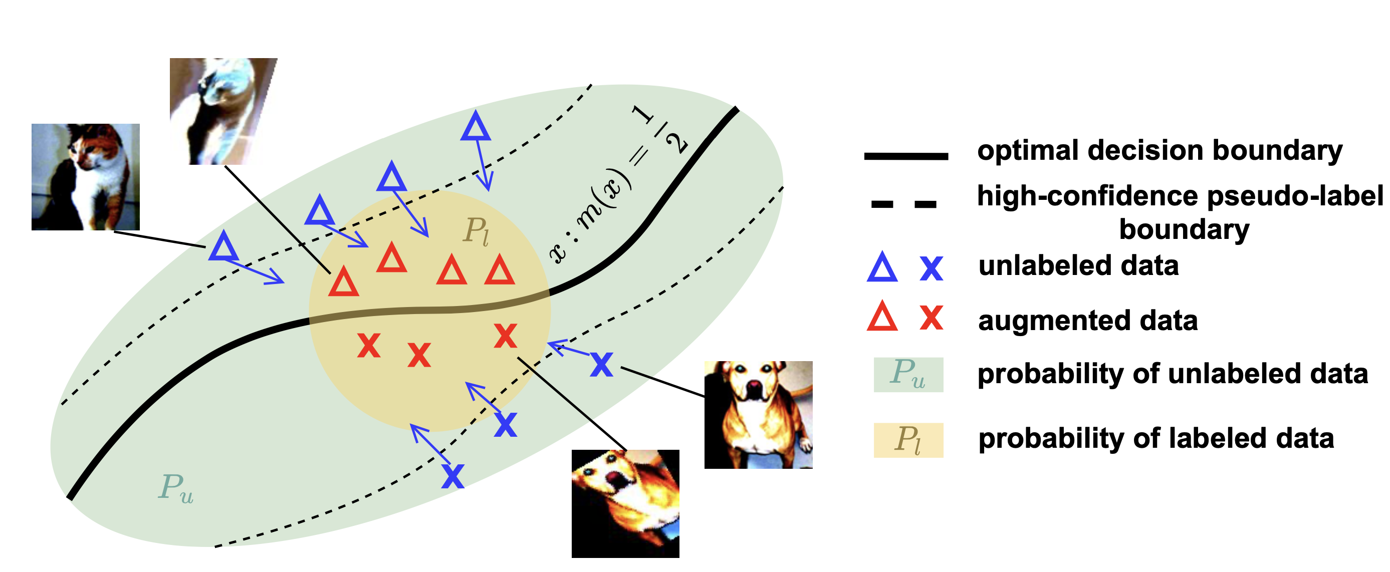
Procedure: Specifically, we select an unlabeled data point from the unlabeled data distribution, which has been assigned a high-confidence pseudo-label. This pseudo-label is treated as the true label. We then apply strong data augmentations to create a transformed input, which is designed to approximate the labeled data distribution and better reflect the test distribution. The pair of strong-augmented input and its original pseudo-label is subsequently treated as labeled data in the training process.

Insights: The valuable information captured from the unlabeled data is transferred to the model in a way that improves its performance on data that might otherwise have been underrepresented or insufficiently trained using the labeled dataset alone.

Next, we revisit the CIFAR10 classification task, but now with only $1000$ labeled images and $49000$ unlabeled images for training.

Let us first import necessary packages and the RandAugment class as borrowed from this repo.

import numpy as np
import random
import torch
from torchvision.utils import make_grid
from torchvision import datasets, models, transforms
import PIL
import PIL.ImageOps
import PIL.ImageEnhance
import PIL.ImageDraw
from PIL import Image
import matplotlib.pyplot as plt

PARAMETER_MAX = 10

def _float_parameter(v, max_v):
    return float(v) * max_v / PARAMETER_MAX

def _int_parameter(v, max_v):
    return int(v * max_v / PARAMETER_MAX)

class RandAugment:
    def __init__(self, n=2, m=10):
        self.n = n
        self.m = m
        self.augment_pool = self.rand_augment_pool()

    def __call__(self, img):
        ops = random.sample(self.augment_pool, self.n)
        for op, max_v, bias in ops:
            if max_v is not None:
                v = np.random.randint(1, self.m)
                img = op(img, v=v, max_v=max_v, bias=bias)
            else:
                img = op(img)
        return img

    def rand_augment_pool(self):
        return [
            (PIL.ImageOps.autocontrast, None, None),
            (self.brightness, 1.8, 0.1),
            (self.color, 1.8, 0.1),
            (self.contrast, 1.8, 0.1),
            (self.cutout, 40, None),
            (PIL.ImageOps.equalize, None, None),
            (PIL.ImageOps.invert, None, None),
            (self.posterize, 4, 0),
            (self.rotate, 30, None),
            (self.sharpness, 1.8, 0.1),
            (self.shear_x, 0.3, None),
            (self.shear_y, 0.3, None),
            (self.solarize, 256, None),
            (self.translate_x, 100, None),
            (self.translate_y, 100, None),
        ]

    def brightness(self, img, v, max_v, bias):
        return PIL.ImageEnhance.Brightness(img).enhance(_float_parameter(v, max_v) + bias)

    def color(self, img, v, max_v, bias):
        return PIL.ImageEnhance.Color(img).enhance(_float_parameter(v, max_v) + bias)

    def contrast(self, img, v, max_v, bias):
        return PIL.ImageEnhance.Contrast(img).enhance(_float_parameter(v, max_v) + bias)

    def cutout(self, img, v, max_v, **kwargs):
        if v == 0:
            return img
        w, h = img.size
        x0 = np.random.uniform(0, w)
        y0 = np.random.uniform(0, h)
        x1 = int(max(0, x0 - v / 2.))
        y1 = int(max(0, y0 - v / 2.))
        x2 = int(min(w, x0 + v))
        y2 = int(min(h, y0 + v))
        img = img.copy()
        PIL.ImageDraw.Draw(img).rectangle((x1, y1, x2, y2), (127, 127, 127))
        return img

    def posterize(self, img, v, max_v, bias):
        return PIL.ImageOps.posterize(img, _int_parameter(v, max_v) + bias)

    def rotate(self, img, v, max_v, **kwargs):
        return img.rotate(_float_parameter(v, max_v))

    def sharpness(self, img, v, max_v, bias):
        return PIL.ImageEnhance.Sharpness(img).enhance(_float_parameter(v, max_v) + bias)

    def shear_x(self, img, v, max_v, **kwargs):
        return img.transform(img.size, PIL.Image.AFFINE, (1, _float_parameter(v, max_v), 0, 0, 1, 0))

    def shear_y(self, img, v, max_v, **kwargs):
        return img.transform(img.size, PIL.Image.AFFINE, (1, 0, 0, _float_parameter(v, max_v), 1, 0))

    def solarize(self, img, v, max_v, **kwargs):
        return PIL.ImageOps.solarize(img, 256 - _int_parameter(v, max_v))

    def translate_x(self, img, v, max_v, **kwargs):
        dx = _float_parameter(v, max_v) * img.size[0]
        return img.transform(img.size, PIL.Image.AFFINE, (1, 0, dx, 0, 1, 0))

    def translate_y(self, img, v, max_v, **kwargs):
        dy = _float_parameter(v, max_v) * img.size[1]
        return img.transform(img.size, PIL.Image.AFFINE, (1, 0, 0, 0, 1, dy))

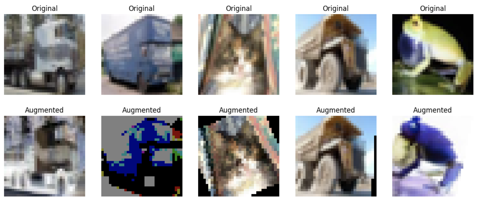
Figure: Visualization of Images Before and After Strong Augmentation

Sample Aug

Define the data loader.

import torch.nn as nn
import torch.optim as optim
from torch.utils.data import DataLoader, Subset, random_split
from sklearn.model_selection import train_test_split

class AugTransform:
    def __init__(self):
        data_stats = ((0.4914, 0.4822, 0.4465), (0.247, 0.243, 0.261))
        self.weak = transforms.Compose([
            transforms.RandomHorizontalFlip(),
            transforms.RandomCrop(32, padding=4, padding_mode='reflect'),
            transforms.ToTensor(),
            transforms.Normalize(*data_stats)
        ])
        self.strong = transforms.Compose([
            transforms.RandomHorizontalFlip(),
            transforms.RandomCrop(32, padding=4, padding_mode='reflect'),
            transforms.RandAugment(),
            transforms.ToTensor(),
            transforms.Normalize(*data_stats)
        ])
        self.identity = transforms.Compose([
            transforms.ToTensor(),
            transforms.Normalize(*data_stats)
        ])
        
    def apply_weak(self, data):
        return self.weak(data)

    def apply_strong(self, data):
        return self.strong(data)

    def apply_identity(self, data):
        return self.identity(data)

class TransformedDataset(torch.utils.data.Dataset):
    def __init__(self, dataset, transform_weak=None, transform_strong=None, mode='train'):
        self.dataset = dataset
        self.transform_weak = transform_weak
        self.transform_strong = transform_strong
        self.mode = mode  # 'train' or 'test'

    def __len__(self):
        return len(self.dataset)

    def __getitem__(self, idx):
        image, label = self.dataset[idx]
        if self.mode == 'train':
            image_weak = self.transform_weak(image) if self.transform_weak else image
            image_strong = self.transform_strong(image) if self.transform_strong else image
            return image_weak, image_strong, label
        elif self.mode == 'test':
            image = self.transform_weak(image) if self.transform_weak else image
            return image, label

# Define augmentation transformer
augmenter = AugTransform()

# Load CIFAR-10 dataset
full_dataset = datasets.CIFAR10('./data', train=True, download=True)
test_dataset = datasets.CIFAR10('./data', train=False, download=True)

# Split dataset into labeled and unlabeled subsets
num_labeled = 1000
labeled_indices, unlabeled_indices = train_test_split(range(len(full_dataset)), train_size=num_labeled, random_state=42)
labeled_dataset = Subset(full_dataset, labeled_indices)
unlabeled_dataset = Subset(full_dataset, unlabeled_indices)

# Creating datasets with transformations applied
transformed_labeled_dataset = TransformedDataset(labeled_dataset, transform_weak=augmenter.apply_weak, transform_strong=augmenter.apply_strong, mode='train')
transformed_unlabeled_dataset = TransformedDataset(unlabeled_dataset, transform_weak=augmenter.apply_weak, transform_strong=augmenter.apply_strong, mode='train')
transformed_test_dataset = TransformedDataset(test_dataset, transform_weak=augmenter.apply_identity, mode='test')

# Data loaders
batch_size = 50
labeled_loader = DataLoader(transformed_labeled_dataset, batch_size=batch_size, shuffle=True)
unlabeled_loader = DataLoader(transformed_unlabeled_dataset, batch_size=batch_size, shuffle=True)
test_loader = DataLoader(transformed_test_dataset, batch_size=batch_size, shuffle=False)

Set up the model.

model = models.resnet18(pretrained=False, num_classes=10)
device = torch.device("cuda" if torch.cuda.is_available() else "cpu")
model.to(device)
optimizer = optim.Adam(model.parameters(), lr=0.001)
criterion = nn.CrossEntropyLoss()

Start training and visualizing of results. The functions evaluate_model and visualize_predictions are the same as those used for supervised learning.

def train(model, labeled_loader, unlabeled_loader, test_loader, optimizer, device, epochs=100, threshold=0.9):
    model.train()
    for epoch in range(epochs):
        total_loss = 0
        total_batches = 0
        total_batch_size = 0  # To track average batch size per epoch

        # Create an iterator for unlabeled data
        unlabeled_iter = iter(unlabeled_loader)

        for labeled_data_weak, _, labels in labeled_loader:
            labeled_data_weak = labeled_data_weak.to(device)
            labels = labels.to(device)
            try:
                # Try to get a batch from unlabeled data
                unlabeled_data_weak, unlabeled_data_strong, _ = next(unlabeled_iter)
                unlabeled_data_weak = unlabeled_data_weak.to(device)
                unlabeled_data_strong = unlabeled_data_strong.to(device)
            except StopIteration:
                # Refresh iterator if the unlabeled loader is exhausted
                unlabeled_iter = iter(unlabeled_loader)
                unlabeled_data_weak, unlabeled_data_strong, _ = next(unlabeled_iter)
                unlabeled_data_weak = unlabeled_data_weak.to(device)
                unlabeled_data_strong = unlabeled_data_strong.to(device)

            # Generate pseudo-labels using weak augmentation
            with torch.no_grad():
                outputs = model(unlabeled_data_weak)
                soft_labels = torch.softmax(outputs, dim=1)
                max_probs, pseudo_labels = torch.max(soft_labels, dim=1)
                mask = max_probs > threshold

            # Generate high-confidence pseudo-labeled data
            if mask.sum() > 0:
                high_conf_data_strong = unlabeled_data_strong[mask]
                high_conf_labels = pseudo_labels[mask].to(device)
            else:
                high_conf_data_strong = torch.tensor([], device=device)
                high_conf_labels = torch.tensor([], dtype=torch.long, device=device)

            # Combine labeled and high-confidence pseudo-labeled data
            combined_data = torch.cat([labeled_data_weak, high_conf_data_strong], dim=0)
            combined_labels = torch.cat([labels, high_conf_labels], dim=0)

            # Forward pass
            outputs = model(combined_data)
            loss = criterion(outputs, combined_labels)

            # Backward pass
            optimizer.zero_grad()
            loss.backward()
            optimizer.step()

            total_loss += loss.item()
            total_batches += 1
            total_batch_size += combined_data.size(0)  # Track total batch size

        average_batch_size = total_batch_size / total_batches
        print(f'Epoch {epoch + 1}, Loss: {total_loss / total_batches}, Avg Batch Size: {average_batch_size}')

        # Visualization and accuracy every few epochs
        if epoch % 20 == 0 or epoch == epochs-1:
            accuracy, predicted = evaluate_model(model, device, test_loader)
            print(f'Epoch {epoch + 1}, Validation accuracy: {accuracy}')
            images, _ = next(iter(test_loader))
            images = images.to(device)
            outputs = model(images)
            _, predicted = torch.max(outputs, 1)
            visualize_predictions(images.cpu(), predicted.cpu().numpy(), class_names)
            
train(model, labeled_loader, unlabeled_loader, test_loader, optimizer, device)

Try the above codes and monitor how the average batch size and accuracy change over time.

Reinforcement Learning¶

Reinforcement Learning (RL) is a type of machine learning where an agent learns to make decisions by performing actions in an environment to maximize some notion of cumulative reward. RL is characterized by:

Agent: Learns from experiences to make decisions.
Environment: Where the agent operates.
Action: A set of decisions the agent can make.
State: The current situation returned by the environment.
Reward: Feedback from the environment to assess the actions.

Policy Gradient Methods¶

Policy Gradient Methods are a class of algorithms in RL that directly optimize the policy, a mapping from states to actions that determines the agent’s actions. Unlike value-based methods that first estimate a value function and derive a policy, policy gradient methods optimize the policy parameters $\theta$ through gradient ascent on the expected return.

Policy Function The policy $\pi_\theta(s, a)$ specifies the probability of selecting action $a$ in state $s$ under a policy parameterized by $\theta$ . The objective in policy gradient methods is to maximize the expected return from the initial state distribution:

$J(\theta) = \mathbb{E}_{\tau \sim \pi_\theta} [R(\tau)]$

where $R(\tau)$ denotes the return of trajectory $\tau$ . The policy is updated by $\theta_{new} = \theta + \alpha \nabla_\theta J(\theta)$ , where $\alpha$ is the learning rate.

Policy Gradient Theorem The gradient of the expected return is given by:

$\nabla_\theta J(\theta) = \mathbb{E}_{\tau \sim \pi_\theta} \left[ \sum_{t=0}^T G_t \nabla_\theta \log \pi_\theta(s_t, a_t) \right]$

Here, $G_t$ represents the total discounted reward from timestep $t$ to the end of the episode, and is calculated as $G_t = \sum_{k=t}^{T} \gamma^{k-t} r_k$ , where $\gamma$ is the discount factor and $r_k$ is the reward received at step $k$ .

Value Function and Advantage Function¶

The value function $V^\pi(s)$ represents the expected return from starting in state $s$ and following policy $\pi$ :

$V^\pi(s) = \mathbb{E}_{\pi} \left[ \sum_{k=0}^\infty \gamma^k r_{t+k} | S_t = s \right]$

Advantage Function $A^{\pi}(s,a)$ measures the benefit of taking a particular action $a$ in state $s$ over the average action at that state under the current policy.

$A^\pi(s_t, a_t) = Q^\pi(s_t, a_t) - V^\pi(s_t) = \mathbb{E}[G_t | S_t = s_t, A_t = a_t, \pi] - V^\pi(s)$

It can be shown that

$\nabla_\theta J(\theta) = \mathbb{E}_{\tau \sim \pi_\theta} \left[ \sum_{t=0}^T A^{\pi_{\theta}}(s_t, a_t) \nabla_\theta \log \pi_\theta(s_t, a_t) \right]$

Generalized Advantage Estimation (GAE) uses the value function to produce a more stable estimator of the advantage function for policy gradients:

$\hat{A}_t = \sum_{k=t}^{T-1} (\gamma \lambda)^{k-t} \delta_k$

where $\delta_k = r_k + \gamma V(s_{k+1}) - V(s_k)$ represents the Temporal Difference (TD) error at step $k$ , and $\lambda$ is a factor that balances bias and variance in the advantage estimation. $T$ denotes the length of the episode.

Proximal Policy Optimization (PPO)¶

PPO, an advanced policy gradient technique, refines basic policy gradient methods by introducing mechanisms like clipping to control policy updates. This is important to prevent drastic changes that lead to unstable training.

PPO Objective Function¶

The objective function for PPO minimizes large updates to the policy by using a clipped surrogate objective:

$L^{CLIP}(\theta) = \hat{\mathbb{E}}_t \left[ \min(r_t(\theta) \hat{A}_t, \text{clip}(r_t(\theta), 1-\epsilon, 1+\epsilon) \hat{A}_t) \right]$

where:

$r_t(\theta) = \frac{\pi_\theta(a_t|s_t)}{\pi_{\theta_{old}}(a_t|s_t)}$ is the probability ratio.
$\hat{A}_t$ is the advantage estimate at timestep $t$ .
$\epsilon$ is a hyperparameter that controls the extent of clipping to prevent drastic updates.

PPO’s using clipped ratios and advantage estimation facilitate stable and efficient policy learning, making it a preferred choice in many practical RL applications.

To calculate $\hat{A}_t$ , we typically simulate a batch of trajectories using the current policy. Each trajectory provides a sequence of states, actions, and rewards from which we compute returns and subsequently advantage estimates, and then perform an update. Neural networks are used in optimizing policies and value functions.

Example: Carpole Game¶

pip install gym moviepy ipython

Note: the following code runs well on Numpy version 1.26, but may give errors on other versions.

import gym
import torch
import torch.nn as nn
import torch.nn.functional as F
import torch.optim as optim
from torch.distributions import Categorical
import numpy as np

class PolicyNet(nn.Module):
    def __init__(self, input_size, output_size, hidden_size=64):
        super(PolicyNet, self).__init__()
        self.fc1 = nn.Linear(input_size, hidden_size)
        self.fc2 = nn.Linear(hidden_size, hidden_size)
        self.fc3 = nn.Linear(hidden_size, output_size)

    def forward(self, x):
        x = F.relu(self.fc1(x))
        x = F.relu(self.fc2(x))
        return torch.softmax(self.fc3(x), dim=-1)

class ValueNet(nn.Module):
    def __init__(self, input_size, hidden_size=64):
        super(ValueNet, self).__init__()
        self.fc1 = nn.Linear(input_size, hidden_size)
        self.fc2 = nn.Linear(hidden_size, hidden_size)
        self.fc3 = nn.Linear(hidden_size, 1)

    def forward(self, x):
        x = F.relu(self.fc1(x))
        x = F.relu(self.fc2(x))
        return self.fc3(x)

class PPOAgent:
    def __init__(self, env, gamma=0.99, lr=1e-3):
        self.env = env
        self.gamma = gamma
        self.device = torch.device("cuda" if torch.cuda.is_available() else "cpu")
        self.policy_net = PolicyNet(env.observation_space.shape[0], env.action_space.n).to(self.device)
        self.value_net = ValueNet(env.observation_space.shape[0]).to(self.device)
        self.policy_optimizer = torch.optim.Adam(self.policy_net.parameters(), lr=lr)
        self.value_optimizer = torch.optim.Adam(self.value_net.parameters(), lr=lr)

        print(f"Initialized agent with state space: {env.observation_space.shape}, action space: {env.action_space.n}")

    def select_action(self, state):

        if isinstance(state, tuple):
            state = state[0]
        elif isinstance(state, dict):
            state = state['observation']
   
        # Ensure state is a NumPy array
        if not isinstance(state, np.ndarray):
            state = np.array(state, dtype=np.float32)

        state_tensor = torch.from_numpy(state).float().unsqueeze(0).to(self.device)
        probs = self.policy_net(state_tensor)
        dist = Categorical(probs)
        action = dist.sample()
        log_prob = dist.log_prob(action)
        value = self.value_net(state_tensor)

        return action.item(), log_prob, value

    def update_policy(self, rewards, log_probs, states, actions, values):
        discounts = [self.gamma ** i for i in range(len(rewards))]

        # Ensure rewards are on the same device
        rewards = torch.tensor(rewards, device=self.device).float()
        R = sum([a * b for a, b in zip(discounts, rewards)])

        policy_loss = []
        value_loss = []
        for log_prob, value, reward in zip(log_probs, values, rewards):
            advantage = R - value.item()
            policy_loss.append(-log_prob * advantage)
            # Ensure R is a tensor on the right device
            value_loss.append(F.smooth_l1_loss(value, torch.tensor([R], device=self.device)))

        # Gradient descent for policy network
        self.policy_optimizer.zero_grad()
        sum(policy_loss).backward()
        self.policy_optimizer.step()

        # Gradient descent for value network
        self.value_optimizer.zero_grad()
        sum(value_loss).backward()
        self.value_optimizer.step()

    def train(self, max_episodes=500):
        for episode in range(max_episodes):
            state = self.env.reset()
            done = False
            log_probs = []
            values = []
            rewards = []
            actions = []
            while not done:
                action, log_prob, value = self.select_action(state)
                step_output = self.env.step(action)
                new_state, reward, done, *_ = step_output
                log_probs.append(log_prob)
                values.append(value)
                rewards.append(reward)
                actions.append(action)
                state = new_state
            self.update_policy(rewards, log_probs, state, actions, values)
            print(f'Episode {episode + 1}, Total reward: {sum(rewards)}')

# Create the environment
env = gym.make('CartPole-v1')

# Create and train the agent
agent = PPOAgent(env)
agent.train()
env.close()

Save trained model.

## making directory
import os
result_dir = os.path.join(os.getcwd(), 'results')
os.makedirs(result_dir, exist_ok=True)
torch.save(agent.policy_net.state_dict(), os.path.join(result_dir, 'ppo_policy_net.pth'))
torch.save(agent.value_net.state_dict(), os.path.join(result_dir, 'ppo_value_net.pth'))
print("Models saved successfully.")

Visualize and save to mp4.

Note: You may encounter the error: AttributeError: 'list' object has no attribute 'shape' in some work environments. To fix this issue, consider changing the line frames.append(frame) to frames.append(frame[0]).

from IPython.display import Video, display
import moviepy.editor as mpy

ddef save_video(frames, filename='gameplay.mp4', fps=30):
    filepath = os.path.join(result_dir, filename)
    clip = mpy.ImageSequenceClip(frames, fps=fps)
    clip.write_videofile(filepath, codec='libx264')
    return filepath

env = gym.make('CartPole-v1', render_mode='rgb_array')
device = torch.device("cuda" if torch.cuda.is_available() else "cpu")
agent = PPOAgent(env)
agent.policy_net.load_state_dict(torch.load(os.path.join(result_dir, 'ppo_policy_net.pth')))
agent.policy_net.to(device)

frames = []
state = env.reset()
for t in range(300):
    frame = env.render()
    frames.append(frame)
    action, _, _ = agent.select_action(state)
    state, reward, done, info, *_ = env.step(action)
    if done:
        break
env.close()

video_path = save_video(frames)
display(Video(video_path, embed=True))

Carpole GIF

References¶

This documentation includes code examples and concepts adapted from the following sources. We acknowledge and thank the authors for their contributions to the open-source community.

SemiFL: Semi-Supervised Federated Learning for Unlabeled Clients with Alternate Training. paper and code
FixMatch: Simplifying Semi-Supervised Learning with Consistency and Confidence. paper
RandAugment: Practical data augmentation with no separate search. code
Intro to Policy Optimization. blog